
Calgary’s September 2026 housing market remained balanced overall, but the city-wide result continues to hide meaningful differences by property type and district. This report uses the September CREB® City of Calgary Monthly Statistics to examine the current dashboard, the 13-month sales, new-listing and inventory trajectory, property-type divergence, and geographic supply conditions.
Executive Summary
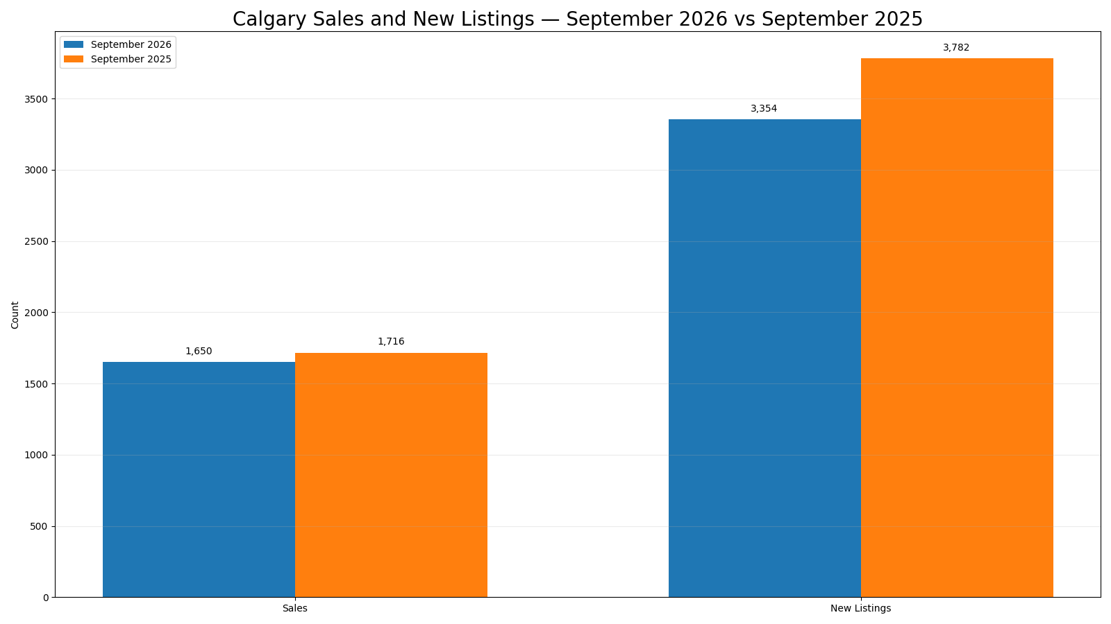
Calgary finished September 2026 in balanced territory with 3.93 months of supply. Sales totalled 1,650, down 3.85% from a year earlier, while 3,354 new listings were 11.32% lower and inventory of 6,486 was 6.26% lower. The benchmark price was $566,700, down 0.82% year over year.
Those headline measures describe a market that has more negotiating room than the tight conditions seen earlier in the cycle, but September did not move uniformly across housing types. Detached and semi-detached sales were higher than a year ago and both remained within balanced supply ranges. Row and apartment sales were lower, with months of supply above four in both segments and larger benchmark-price declines, especially for apartments. Geography adds another layer: the district-by-property-type matrix shows that supply can differ sharply within the same part of Calgary.
For buyers and sellers, the practical implication is that a single city-wide market label is not enough to judge competition. Property type, district and the specific pool of comparable listings matter. The next useful signals are whether inventory continues to ease after its summer peak, whether sales stabilize into the autumn, and whether the higher-supply row and apartment segments begin to narrow their supply and price differences relative to the lower-supply segments.
Calgary Market at a Glance
How Market Conditions Are Changing
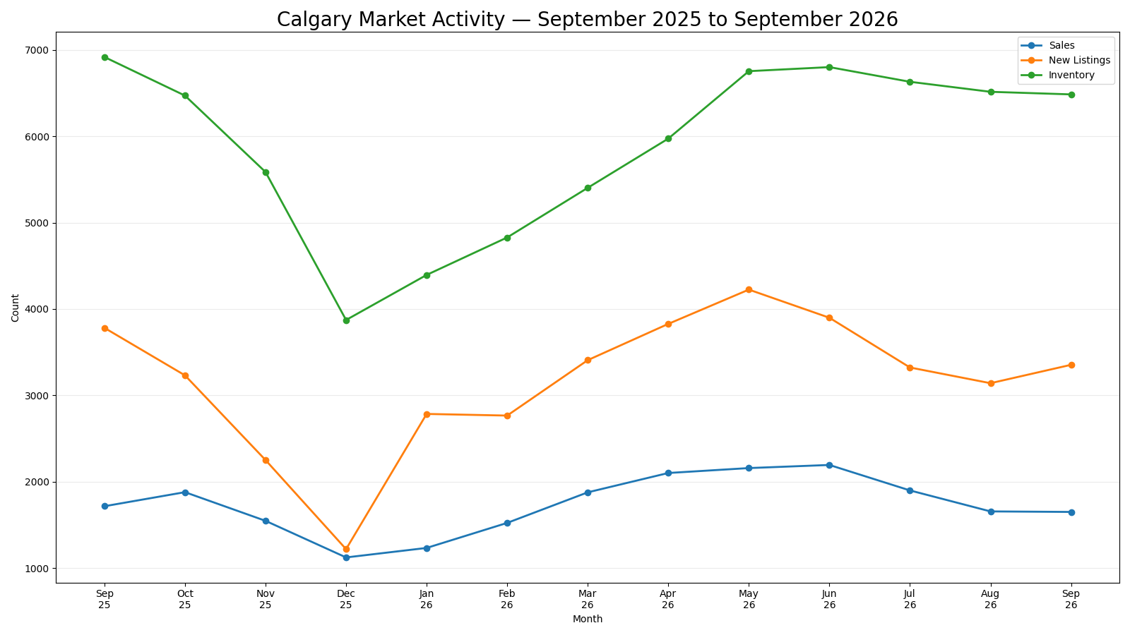
The 13-month trajectory shows a market that expanded materially through the first half of 2026 and then eased into September. Sales rose from 1,233 in January to a June high of 2,194 before slowing to 1,899 in July, 1,656 in August and 1,650 in September. New listings followed a similar seasonal expansion, reaching 4,225 in May and remaining elevated through June before moving lower in July and August. September new listings increased from August to 3,354, but they were still 11.32% below September 2025.
Inventory accumulated as the spring market progressed, climbing from 4,395 in January to 6,802 in June. It then declined modestly through the summer and stood at 6,486 in September, 6.26% below the prior-year level. That combination matters because market competitiveness depends on how demand and available supply move together, not on either measure in isolation. September’s 3.93 months of supply remained within the governed balanced range, but it sat close to the upper boundary. The benchmark price of $566,700 was 0.82% below a year earlier and days on market increased to 44 from 42.
Together, these measures indicate a market with enough supply to limit broad upward price pressure while still avoiding an overall city-wide buyer’s-market classification. The main change since spring is therefore not a collapse in activity, but a transition from stronger seasonal sales toward slower autumn demand while inventory remains substantial. Whether that balance tightens or loosens further will depend on the relative pace of sales and listing absorption over the next several months. Reading the full sequence also prevents a single monthly change from being mistaken for the entire trend, because the current supply position reflects the cumulative movement of sales, listings and inventory across the year.
Where the Market Is Diverging
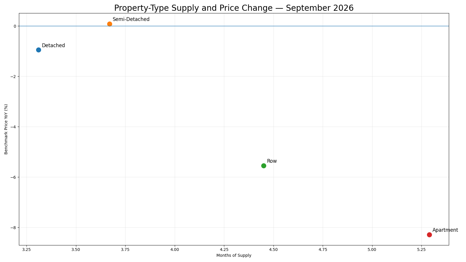
The city-wide result masks a clear split between lower-density and higher-density property types. Semi-detached homes recorded the strongest year-over-year sales change at +5.16%, with 3.67 months of supply and a benchmark price that was essentially unchanged at +0.09% year over year. Detached sales were also higher, up 4.43%, while inventory was 7.28% lower and months of supply measured 3.31. Its benchmark price was down a comparatively modest 0.95%.
Row and apartment properties showed a different pattern. Row sales fell 18.15% from a year earlier while inventory edged 0.73% higher, producing 4.45 months of supply and a 5.54% benchmark-price decline. Apartment sales were down 14.25%; inventory was also lower year over year, but supply remained the highest of the four property types at 5.29 months. The apartment benchmark price declined 8.28%, the largest decrease among the four segments.
This is not a simple story of inventory rising everywhere. Apartment inventory was 9.38% below a year earlier, yet weaker sales were still sufficient to leave the segment with the most supply relative to demand. Conversely, detached and semi-detached markets combined positive sales growth with lower inventory and remained in balanced territory. The divergence therefore comes from the interaction of sales, available inventory and the rate at which that inventory is being absorbed. Calgary’s overall 3.93 months of supply is a useful reference point, but it sits between materially different segment conditions. Buyers and sellers evaluating a specific property should therefore avoid treating the city-wide figure as a direct proxy for the competition affecting detached, semi-detached, row or apartment homes.
The four indicators should be read as a combined evidence set rather than ranked independently, because each describes a different part of the current market balance. Sales change measures demand relative to last year, inventory change measures available stock, months of supply relates that stock to the sales pace, and benchmark-price change records the resulting price direction without establishing causation. A segment can therefore have falling inventory and still carry more supply relative to demand when sales have weakened enough, just as stronger sales can offset a sizeable listing pool.
This is why the comparison table retains all four measures instead of reducing each property type to one headline number. The evidence is most informative where several indicators point in the same direction, but mixed signals remain important and should not be forced into a simpler narrative.
| Property Type | Sales YoY | Inventory YoY | Months of Supply | Benchmark Price YoY |
|---|---|---|---|---|
| Detached | +4.43% | -7.28% | 3.31 | -0.95% |
| Semi-Detached | +5.16% | -3.23% | 3.67 | +0.09% |
| Row | -18.15% | +0.73% | 4.45 | -5.54% |
| Apartment | -14.25% | -9.38% | 5.29 | -8.28% |
Geographic Differences
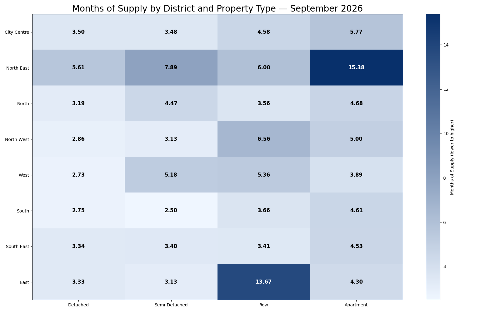
Geographic variation is substantial, but the matrix also shows why district conditions should not be reduced to one label. In North East Calgary, for example, apartment supply reached 15.38 months while detached supply was 5.61 months; both were elevated, but by very different degrees. East Calgary also showed a pronounced contrast, with row supply at 13.67 months compared with 3.13 months for semi-detached and 3.33 months for detached. By comparison, South Calgary had relatively compressed supply across detached, semi-detached and row homes, ranging from 2.50 to 3.66 months, while apartments were higher at 4.61. The West and North West districts likewise show that one property type can diverge from another within the same geography.
These differences matter because city-wide and even district-wide averages can conceal the competitive environment surrounding a specific home. The full matrix is therefore most useful as a map of where supply differs by both location and housing form, rather than as a basis for assigning a single market condition to each district. The exact values remain available in the matrix so readers can verify the local contrast without relying on broad district labels or colour alone.
| District | Detached | Semi-Detached | Row | Apartment |
|---|---|---|---|---|
| City Centre | 3.50 | 3.48 | 4.58 | 5.77 |
| North East | 5.61 | 7.89 | 6.00 | 15.38 |
| North | 3.19 | 4.47 | 3.56 | 4.68 |
| North West | 2.86 | 3.13 | 6.56 | 5.00 |
| West | 2.73 | 5.18 | 5.36 | 3.89 |
| South | 2.75 | 2.50 | 3.66 | 4.61 |
| South East | 3.34 | 3.40 | 3.41 | 4.53 |
| East | 3.33 | 3.13 | 13.67 | 4.30 |
What Is Driving the Market
The September evidence points to an internal market mechanism centred on the balance between sales and available supply. City-wide sales were lower than a year ago, but new listings and inventory were also lower, limiting the extent to which months of supply expanded. At the property-type level, the same relationship explains much of the divergence. Detached and semi-detached demand held up better year over year while inventory was lower, keeping their months of supply within balanced ranges. Row demand weakened while inventory was slightly higher, and apartment demand weakened enough that supply remained elevated even though inventory itself was lower.
The resulting benchmark-price changes line up with those relative supply conditions without proving that months of supply alone caused the price movements. The district matrix reinforces the same point: different combinations of sales and inventory create substantially different supply positions by housing type and location. This report does not use the governed data to attribute those patterns to interest rates, migration, construction, policy or other external factors. The evidence supports an interpretation of changing market balance; it does not, by itself, establish the external causes behind that change.
What This Means for Buyers and Sellers
For buyers, the September data suggest that negotiating conditions depend heavily on property type and location. The city-wide market remains balanced, but row and apartment properties carry more months of supply than detached and semi-detached homes. That can translate into a broader set of competing listings and more opportunity to compare condition, pricing and time on market before committing. It does not mean every row home or apartment will be weakly contested: district-level supply varies widely, and well-positioned properties can still attract competition. Buyers should therefore compare a candidate home with current alternatives in its own segment and district rather than relying solely on the Calgary-wide dashboard.
For sellers, balanced city-wide conditions place more emphasis on accurate positioning. Detached and semi-detached segments are showing stronger sales performance than row and apartment segments, but neither is uniformly tight across all districts. Sellers in higher-supply segments face a clearer need to understand the active competition and the recent benchmark direction for their property type. In practical terms, pricing above the evidence supplied by comparable listings can create additional exposure time when buyers have more choice. Sellers in lower-supply pockets may have stronger relative positioning, but the data do not support assuming a uniform seller’s market.
For both sides, the most useful framework is hierarchical: start with the city-wide context, then narrow to property type, district, and finally comparable listings. That approach better reflects the divergence visible in September and reduces the risk of applying a broad market narrative to a local decision where the competitive set is materially different. The practical difference is a matter of market context rather than a forecast: more available choice can strengthen a buyer’s ability to compare alternatives, while tighter local supply can increase the importance of preparation and timely decisions. Neither condition guarantees a particular negotiating outcome, because individual property quality, pricing and the immediate comparable set still determine how a specific listing competes.
What to Watch Next
Three relationships are worth monitoring next. First, watch whether city-wide inventory continues to decline from the summer peak while sales stabilize. A faster inventory decline relative to sales would tend to tighten months of supply; renewed inventory growth without comparable sales growth would do the opposite. Second, watch the gap between detached/semi-detached conditions and row/apartment conditions.
A sustained reduction in row and apartment months of supply would indicate that the current property-type divergence is narrowing. Third, watch district-level supply in the areas with the largest September extremes, particularly apartment supply in the North East and row supply in the East. Material movement there would show whether today’s geographic outliers are temporary or persisting. These are monitoring conditions rather than forecasts: the next reports should be evaluated against the same official CREB measures to determine whether the current balance is changing.
Explore the Market in More Detail
Sources and Methodology
Quantitative evidence in this September 2026 report comes from the official CREB® City of Calgary Monthly Statistics package. Sales, New Listings, Inventory, Months of Supply, benchmark prices, the 13-month trajectory, property-type comparison and district-by-property-type supply matrix all use CREB-published values. Market Status is derived from official months of supply using the report framework: below 2.5 months is a Seller’s Market, 2.5 to 4.0 is a Balanced Market, and above 4.0 is a Buyer’s Market.